Data types#
AiiDA already ships with a number of useful data types. This section details the most common, and some handy features/functionalities to work with them.
The different data types can be accessed through the DataFactory() function (also exposed from aiida.plugins) by passing the corresponding entry point as an argument, for example when working in the verdi shell:
In [1]: ArrayData = DataFactory('core.array')
Important
Many of the examples in this section will assume you are working inside the verdi shell.
If this is not the case, you will have to first load e.g. the DataFactory() function:
from aiida.plugins import DataFactory

ArrayData = DataFactory('core.array')
A list of all the data entry points can be obtain running the command verdi plugin list aiida.data.
For all data types, you can follow the link to the corresponding data class in the API reference to read more about the class and its methods. We also detail what is stored in the database (mostly as attributes, so the information can be easily queried e.g. with the QueryBuilder) and what is stored as a raw file in the AiiDA file repository (providing access to the file contents, but not efficiently queryable: this is useful for e.g. big data files that don’t need to be queried for).
If you need to work with some specific type of data, first check the list of data types/plugins below, and if you don’t find what you need, give a look to Adding support for custom data types.
Core data types#
Below is a list of the core data types already provided with AiiDA, along with their entry point and where the data is stored once the node is stored in the AiiDA database.
Class |
Entry point |
Stored in database |
Stored in repository |
|---|---|---|---|
|
The integer value |
\- |
|
|
The float value |
\- |
|
|
The string |
\- |
|
|
The boolean value |
\- |
|
|
The complete list |
\- |
|
|
The complete dictionary |
\- |
|
|
The value, name and the class identifier |
\- |
|
|
The JSON data and the class identifier |
\- |
|
|
The array names and corresponding shapes |
The array data in |
|
|
The array names and corresponding shapes |
The array data in |
|
|
The filename |
The file |
|
|
\- |
All files and folders |
|
|
The computer and the absolute path to the folder |
All files and folders |
Base types#
There are a number of useful classes that wrap base Python data types (Int, Float, Str, Bool) so they can be stored in the provenance.
These are automatically loaded with the verdi shell, and also directly exposed from aiida.orm.
They are particularly useful when you need to provide a single parameter to e.g. a workfunction.
Each of these classes can most often be used in a similar way as their corresponding base type:
In [1]: total = Int(2) + Int(3)
If you need to access the bare value and not the whole AiiDA class, use the .value property:
In [2]: total.value
Out[2]: 5
Warning
While this is convenient if you need to do simple manipulations like multiplying two numbers, be very careful not to pass such nodes instead of the corresponding Python values to libraries that perform heavy computations with them. In fact, any operation on the value would be replaced with an operation creating new AiiDA nodes, that however can be orders of magnitude slower (see this discussion on GitHub). In this case, remember to pass the node.value to the mathematical function instead.
AiiDA has also implemented data classes for two basic Python iterables: List and Dict. They can store any list or dictionary where elements can be a base python type (strings, floats, integers, booleans, None type):
In [1]: l = List(list=[1, 'a', False])
Note the use of the keyword argument list, this is required for the constructor of the List class.
You can also store lists or dictionaries within the iterable, at any depth level.
For example, you can create a dictionary where a value is a list of dictionaries:
In [2]: d = Dict(dict={'k': 0.1, 'l': [{'m': 0.2}, {'n': 0.3}]})
To obtain the Python list or dictionary from a List or Dict instance, you have to use the get_list() or get_dict() methods:
In [3]: l.get_list()
Out[3]: [1, 'a', False]

In [4]: d.get_dict()
Out[4]: {'k': 0.1, 'l': [{'m': 0.2}, {'n': 0.3}]}
However, you can also use the list index or dictionary key to extract specific values:
In [5]: l[1]
Out[5]: 'a'

In [6]: d['k']
Out[6]: 0.1
You can also use many methods of the corresponding Python base type, for example:
In [7]: l.append({'b': True})

In [8]: l.get_list()
Out[8]: [1, 'a', False, {'b': True}]
For all of the base data types, their value is stored in the database in the attributes column once you store the node using the store() method.
EnumData#
New in version 2.0.
An Enum member is represented by three attributes in the EnumData class:
name: the member’s namevalue: the member’s valueidentifier: the string representation of the enum’s identifier
In [1]: from enum import Enum
   ...: class Color(Enum):
   ...: RED = 1
   ...: GREEN = 2

In [2]: from aiida.orm import EnumData
   ...: color = EnumData(Color.RED)

In [3]: color.name
Out[3]: 'RED'

In [4]: color.value
Out[4]: 1

In [5]: color.get_member()
Out[5]: <Color.RED: 1>
JsonableData#
New in version 2.0.
JsonableData is a data plugin that allows one to easily wrap existing objects that are JSON-able.
Any class that implements an as_dict method, returning a dictionary that is a JSON serializable representation of the object, can be wrapped and stored by this data plugin.
To deserialize it should also implement a from_dict method, which takes the dictionary as input and returns the object.
In [1]: from aiida.orm import JsonableData
   ...: class MyClass:
   ...:     def __init__(self, a: int, b: int):
   ...:         self.a = a
   ...:         self.b = b
   ...:     def __str__(self):
   ...:         return f'MyClass({self.a}, {self.b})'
   ...:     def as_dict(self) -> dict:
   ...:         return {'a': self.a, 'b': self.b}
   ...:     @classmethod
   ...:     def from_dict(cls, d: dict):
   ...:         return cls(d['a'], d['b'])
   ...:
   ...: my_object = MyClass(1, 2)
   ...: my_jsonable = JsonableData(my_object)
   ...: str(my_jsonable.obj)
Out[1]: 'MyClass(1, 2)'
ArrayData#
The ArrayData class can be used to represent numpy arrays in the provenance.
Each array is assigned to a name specified by the user using the set_array() method:
In [1]: ArrayData = DataFactory('core.array'); import numpy as np

In [2]: array = ArrayData()

In [3]: array.set_array('matrix', np.array([[1, 2], [3, 4]]))
Note that one ArrayData instance can store multiple arrays under different names:
In [4]: array.set_array('vector', np.array([[1, 2, 3, 4]]))
To see the list of array names stored in the ArrayData instance, you can use the get_arraynames() method:
In [5]: array.get_arraynames()
Out[5]: ['matrix', 'vector']
If you want the array corresponding to a certain name, simply supply the name to the get_array() method:
In [6]: array.get_array('matrix')
Out[6]:
array([[1, 2],
      [3, 4]])
As with all nodes, you can store the ArrayData node using the store() method. However, only the names and shapes of the arrays are stored to the database, the content of the arrays is stored to the repository in the numpy format (.npy).
XyData#
In case you are working with arrays that have a relationship with each other, i.e. y as a function of x, you can use the XyData class:
In [1]: XyData = DataFactory('core.array.xy'); import numpy as np

In [2]: xy = XyData()
This class is equipped with setter and getter methods for the x and y values specifically, and takes care of some validation (e.g. check that they have the same shape).
The user also has to specify the units for both x and y:
In [3]: xy.set_x(np.array([10, 20, 30, 40]), 'Temperate', 'Celsius')

In [4]: xy.set_y(np.array([1, 2, 3, 4]), 'Volume Expansion', '%')
Note that you can set multiple y values that correspond to the x grid.
Same as for the ArrayData, the names and shapes of the arrays are stored to the database, the content of the arrays is stored to the repository in the numpy format (.npy).
SinglefileData#
In order to include a single file in the provenance, you can use the SinglefileData class.
This class can be initialized via the absolute path to the file you want to store:
In [1]: SinglefileData = DataFactory('core.singlefile')

In [2]: single_file = SinglefileData('/absolute/path/to/file')
The contents of the file in string format can be obtained using the get_content() method:
In [3]: single_file.get_content()
Out[3]: 'The file content'
When storing the node, the filename is stored in the database and the file itself is copied to the repository.
FolderData#
The FolderData class stores sets of files and folders (including its subfolders).
To store a complete directory, simply use the tree keyword:
In [1]: FolderData = DataFactory('core.folder')

In [2]: folder = FolderData(tree='/absolute/path/to/directory')
Alternatively, you can construct the node first and then use the various repository methods to add objects from directory and file paths:
In [1]: folder = FolderData()

In [2]: folder.put_object_from_tree('/absolute/path/to/directory')

In [3]: folder.put_object_from_file('/absolute/path/to/file1.txt', path='file1.txt')
or from file-like objects:
In [4]: folder.put_object_from_filelike(filelike_object, path='file2.txt')
Inversely, the content of the files stored in the FolderData node can be accessed using the get_object_content() method:
In [5]: folder.get_object_content('file1.txt')
Out[5]: 'File 1 content\n'
To see the files that are stored in the FolderData, you can use the list_object_names() method:
In [6]: folder.list_object_names()
Out[6]: ['subdir', 'file1.txt', 'file2.txt']
In this example, subdir was a sub directory of /absolute/path/to/directory, whose contents where added above.
to list the contents of the subdir directory, you can pass its path to the list_object_names() method:
In [7]: folder.list_object_names('subdir')
Out[7]: ['file3.txt', 'module.py']
The content can once again be shown using the get_object_content() method by passing the correct path:
In [8]: folder.get_object_content('subdir/file3.txt')
Out[8]: 'File 3 content\n'
Since the FolderData node is simply a collection of files, it simply stores these files in the repository.
RemoteData#
The RemoteData node represents a “symbolic link” to a specific folder on a remote computer.
Its main use is to allow users to persist the provenance when e.g. a calculation produces data in a raw/scratch folder, and the whole folder needs to be provided to restart/continue.
To create a RemoteData instance, simply pass the remote path to the folder and the computer on which it is stored:
In [1]: RemoteData = DataFactory('core.remote')

In [2]: computer = load_computer(label='computer_label')

In [3]: remote = RemoteData(remote_path='/absolute/path/to/remote/directory' computer=local)
You can see the contents of the remote folder by using the listdir() method:
In [4]: remote.listdir()
Out[4]: ['file2.txt', 'file1.txt', 'subdir']
To see the contents of a subdirectory, pass the relative path to the listdir() method:
In [5]: remote.listdir('subdir')
Out[5]: ['file3.txt', 'module.py']
Warning
Using the listdir() method, or any method that retrieves information from the remote computer, opens a connection to the remote computer using its transport type.
Their use is strongly discouraged when writing scripts and/or workflows.
Materials science data types#
Since AiiDA was first developed within the computational materials science community, aiida-core still contains several data types specific to this field. This sections lists these data types and provides some important examples of their usage.
Class |
Entry point |
Stored in database |
Stored in repository |
|---|---|---|---|
|
The cell, periodic boundary conditions, atomic positions, species and kinds. |
\- |
|
|
The structure species and the shape of the cell, step and position arrays. |
The array data in numpy format. |
|
|
The MD5 of the UPF and the element of the pseudopotential. |
The pseudopotential file. |
|
|
(as mesh) The mesh and offset. (as list) The “kpoints” array shape, labels and their indices. |
\- The array data in numpy format. |
|
|
The units, labels and their numbers, and shape of the bands and kpoints arrays. |
The array data in numpy format. |
StructureData#
The StructureData data type represents a structure, i.e. a collection of sites defined in a cell.
The boundary conditions are periodic by default, but can be set to non-periodic in any direction.
As an example, say you want to create a StructureData instance for bcc Li.
Let’s begin with creating the instance by defining its unit cell:
In [1]: StructureData = DataFactory('core.structure')

In [2]: unit_cell = [[3.0, 0.0, 0.0], [0.0, 3.0, 0.0], [0.0, 0.0, 3.0]]

In [3]: structure = StructureData(cell=unit_cell)
Note
Default units for crystal structure cell and atomic coordinates in AiiDA are Å (Ångström).
Next, you can add the Li atoms to the structure using the append_atom() method:
In [4]: structure.append_atom(position=(0.0, 0.0, 0.0), symbols="Li")

In [5]: structure.append_atom(position=(1.5, 1.5, 1.5), symbols="Li")
You can check if the cell and sites have been set up properly by checking the cell and sites properties:
In [6]: structure.cell
Out[6]: [[3.5, 0.0, 0.0], [0.0, 3.5, 0.0], [0.0, 0.0, 3.5]]

In [7]: structure.sites
Out[7]: [<Site: kind name 'Li' @ 0.0,0.0,0.0>, <Site: kind name 'Li' @ 1.5,1.5,1.5>]
From the StructureData node you can also obtain the formats of well-known materials science Python libraries such as the Atomic Simulation Environment (ASE) and pymatgen:
In [8]: structure.get_ase()
Out[8]: Atoms(symbols='Li2', pbc=True, cell=[3.5, 3.5, 3.5], masses=...)

In [9]: structure.get_pymatgen()
Out[9]:
Structure Summary
Lattice
    abc : 3.5 3.5 3.5
angles : 90.0 90.0 90.0
volume : 42.875
      A : 3.5 0.0 0.0
      B : 0.0 3.5 0.0
      C : 0.0 0.0 3.5
PeriodicSite: Li (0.0000, 0.0000, 0.0000) [0.0000, 0.0000, 0.0000]
PeriodicSite: Li (1.5000, 1.5000, 1.5000) [0.4286, 0.4286, 0.4286]
See also
JsonableData, which can store any other Pymatgen class.
Exporting#
The following export formats are available for StructureData:
xsf(format supported by e.g. XCrySDen and other visualization software; supports periodic cells)xyz(classical xyz format, does not typically support periodic cells (even if the cell is indicated in the comment line)cif(export to CIF format, without symmetry reduction, i.e. always storing the structure as P1 symmetry)
The node can be exported using the verdi CLI, for example:
$ verdi data structure export --format xsf <IDENTIFIER> > Li.xsf
Where <IDENTIFIER> is one of the possible identifiers of the node, e.g. its PK or UUID.
This outputs the structure in xsf format and writes it to a file.
TrajectoryData#
The TrajectoryData data type represents a sequences of StructureData objects, where the number of atomic kinds and sites does not change over time.
Beside the coordinates, it can also optionally store velocities.
If you have a list of StructureData instances called structure_list that represent the trajectory of your system, you can create a TrajectoryData instance from this list:
In [1]: TrajectoryData = DataFactory('core.array.trajectory')

In [2]: trajectory = TrajectoryData(structure_list)
Note that contrary with the StructureData data type, the cell and atomic positions are stored a numpy array in the repository and not in the database.
Exporting#
You can export the py:class:~aiida.orm.nodes.data.array.trajectory.TrajectoryData node with verdi data trajectory export, which accepts a number of formats including xsf and cif, and additional parameters like --step NUM (to choose to export only a given trajectory step).
The following export formats are available:
xsf(format supported by e.g. XCrySDen and other visualization software; supports periodic cells)cif(export to CIF format, without symmetry reduction, i.e. always storing the structures as P1 symmetry)
UpfData#
The UpfData data type represents a pseudopotential in the .UPF format (e.g. used by Quantum ESPRESSO - see also the AiiDA Quantum ESPRESSO plugin).
Usually these will be installed as part of a pseudopotential family, for example via the aiida-pseudo package.
To see the pseudopotential families that have been installed in your AiiDA profile, you can use the verdi CLI:
$ verdi data upf listfamilies
Success: * SSSP_v1.1_precision_PBE [85 pseudos]
Success: * SSSP_v1.1_efficiency_PBE [85 pseudos]
KpointsData#
The KpointsData data type represents either a grid of k-points (in reciprocal space, for crystal structures), or explicit list of k-points (optionally with a weight associated to each one).
To create a KpointsData instance that describes a regular (2 x 2 x 2) mesh of k-points, execute the following set of commands in the verdi shell:
In [1]: KpointsData = DataFactory('core.array.kpoints')
   ...: kpoints_mesh = KpointsData()
   ...: kpoints_mesh.set_kpoints_mesh([2, 2, 2])
This will create a (2 x 2 x 2) mesh centered at the Gamma point (i.e. without offset).
Alternatively, you can also define a KpointsData node from a list of k-points using the set_kpoints() method:
In [2]: kpoints_list = KpointsData()
   ...: kpoints_list.set_kpoints([[0, 0, 0], [0.5, 0.5, 0.5]])
In this case, you can also associate labels to (some of the) points, which is very useful for generating plots of the band structure (and storing them in a BandsData instance):
In [3]: kpoints_list.labels = [[0, "G"]]

In [4]: kpoints_list.labels
Out[4]: [(0, 'G')]
Automatic computation of k-point paths#
AiiDA provides a number of tools and wrappers to automatically compute k-point paths given a cell or a crystal structure.
The main interface is provided by the two methods aiida.tools.data.array.kpoints.main.get_kpoints_path() and aiida.tools.data.array.kpoints.main.get_explicit_kpoints_path().
These methods are also conveniently exported directly as, e.g., aiida.tools.get_kpoints_path.
The difference between the two methods is the following:
get_kpoints_path()returns a dictionary of k-point coordinates (e.g.{'GAMMA': [0. ,0. ,0. ], 'X': [0.5, 0., 0.], 'L': [0.5, 0.5, 0.5]}, and then a list of tuples of endpoints of each segment, e.g.[('GAMMA', 'X'), ('X', 'L'), ('L', 'GAMMA')]for the \(\Gamma-X-L-\Gamma\) path.get_explicit_kpoints_path(), instead, returns a list of kpoints that follow that path, with some predefined (but user-customizable) distance between points, e.g. something like[[0., 0., 0.], [0.05, 0., 0.], [0.1, 0., 0.], ...].
Depending on how the underlying code works, one method might be preferred on the other.
The docstrings of the methods describe the expected parameters.
The general interface requires always a StructureData as the first parameter structure, as well as a string for the method to use (by default this is seekpath, but also the legacy method implemented in earlier versions of AiiDA is available; see description below).
Additional parameters are passed as kwargs to the underlying implementation, that often accepts a different number of parameters.
Seekpath implementation#
When specifying method='seekpath', the seekpath library is used to generate the path.
Note that this requires seekpath to be installed (this is not available by default, in order to reduce the dependencies of AiiDA core, but can be easily installed using pip install seekpath).
For a full description of the accepted parameters, we refer to the docstring of the underlying methods aiida.tools.data.array.kpoints.seekpath.get_explicit_kpoints_path() and aiida.tools.data.array.kpoints.seekpath.get_kpoints_path(), and for more general information to the seekpath documentation.
If you use this implementation, please cite the Hinuma paper:
Y. Hinuma, G. Pizzi, Y. Kumagai, F. Oba, I. Tanaka,
Band structure diagram paths based on crystallography,
Comp. Mat. Sci. 128, 140 (2017)
DOI: 10.1016/j.commatsci.2016.10.015
Legacy implementation
This refers to the implementation that has been available since the early versions of AiiDA.
Note
In the 3D case (all three directions have periodic boundary conditions), this implementation expects that the structure is already standardized according to the Setyawan paper (see journal reference below). If this is not the case, the kpoints and band structure returned will be incorrect. The only case that is dealt correctly by the library is the case when axes are swapped, where the library correctly takes this swapping/rotation into account to assign kpoint labels and coordinates.
We therefore suggest that you use the seekpath implementation, that is able to automatically correctly identify the standardized crystal structure (primitive and conventional) as described in the Hinuma paper.
For a full description of the accepted parameters, we refer to the docstring of the underlying methods aiida.tools.data.array.kpoints.legacy.get_explicit_kpoints_path() and aiida.tools.data.array.kpoints.legacy.get_kpoints_path(), and for more general information to the seekpath documentation.
If you use this implementation, please cite the correct reference from the following ones:
The 3D implementation is based on the Setyawan paper:
W. Setyawan, S. Curtarolo,
High-throughput electronic band structure calculations: Challenges and tools,
Comp. Mat. Sci. 49, 299 (2010)
DOI: 10.1016/j.commatsci.2010.05.010
The 2D implementation is based on the Ramirez paper:
R. Ramirez and M. C. Bohm,
Simple geometric generation of special points in brillouin-zone integrations. Two-dimensional bravais lattices
Int. J. Quant. Chem., XXX, 391-411 (1986)
DOI: 10.1002/qua.560300306
BandsData#
The BandsData data type is dedicated to store band structures of different types (electronic bands, phonons, or any other band-structure-like quantity that is a function of the k-points in the Brillouin zone).
In this section we describe the usage of the BandsData to store the electronic band structure of silicon and some logic behind its methods.
The dropdown panels below explain some expanded use cases on how to create a BandsData node and plot the band structure.
Creating a BandsData instance manually
To start working with the BandsData data type we should import it using the DataFactory and create an object of type BandsData:
from aiida.plugins import DataFactory
BandsData = DataFactory('core.array.bands')
bands_data = BandsData()
To import the bands we need to make sure to have two arrays: one containing kpoints and another containing bands.
The shape of the kpoints object should be nkpoints * 3, while the shape of the bands should be nkpoints * nstates.
Let’s assume the number of kpoints is 12, and the number of states is 5.
So the kpoints and the bands array will look as follows:
import numpy as np
kpoints = np.array(
      [[0.    , 0.    , 0.    ], # array shape is 12 * 3
      [0.1   , 0.    , 0.1   ],
      [0.2   , 0.    , 0.2   ],
      [0.3   , 0.    , 0.3   ],
      [0.4   , 0.    , 0.4   ],
      [0.5   , 0.    , 0.5   ],
      [0.5   , 0.    , 0.5   ],
      [0.525 , 0.05  , 0.525 ],
      [0.55  , 0.1   , 0.55  ],
      [0.575 , 0.15  , 0.575 ],
      [0.6   , 0.2   , 0.6   ],
      [0.625 , 0.25  , 0.625 ]])

bands = np.array(
  [[-5.64024889,  6.66929678,  6.66929678,  6.66929678,  8.91047649], # array shape is 12 * 5, where 12 is the size of the kpoints mesh
  [-5.46976726,  5.76113772,  5.97844699,  5.97844699,  8.48186734],  # and 5 is the numbe of states
  [-4.93870761,  4.06179965,  4.97235487,  4.97235488,  7.68276008],
  [-4.05318686,  2.21579935,  4.18048674,  4.18048675,  7.04145185],
  [-2.83974972,  0.37738276,  3.69024464,  3.69024465,  6.75053465],
  [-1.34041116, -1.34041115,  3.52500177,  3.52500178,  6.92381041],
  [-1.34041116, -1.34041115,  3.52500177,  3.52500178,  6.92381041],
  [-1.34599146, -1.31663872,  3.34867603,  3.54390139,  6.93928289],
  [-1.36769345, -1.24523403,  2.94149041,  3.6004033 ,  6.98809593],
  [-1.42050683, -1.12604118,  2.48497007,  3.69389815,  7.07537154],
  [-1.52788845, -0.95900776,  2.09104321,  3.82330632,  7.20537566],
  [-1.71354964, -0.74425095,  1.82242466,  3.98697455,  7.37979746]])
To insert kpoints and bands in the bands_data object we should employ set_kpoints() and set_bands() methods:
bands_data.set_kpoints(kpoints)
bands_data.set_bands(bands, units='eV')
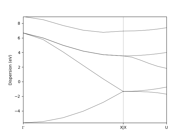
Plotting the band structure
Next we want to visualize the band structure. Before doing so, one thing that we may want to add is the array of kpoint labels:
labels = [(0, 'GAMMA'),
          (5, 'X'),
          (6, 'X'),
          (11, 'U')]

bands_data.labels = labels
bands_data.show_mpl() # to visualize the bands
The resulting band structure will look as follows
Warning
As with any AiiDA node, once the bands_data object is stored (bands_data.store()) it won’t accept any modifications.
You may notice that depending on how you assign the kpoints labels the output of the show_mpl() method looks different.
Please compare:
bands_data.labels = [(0, 'GAMMA'),
          (5, 'X'),
          (6, 'Y'),
          (11, 'U')]
bands_data.show_mpl()

bands_data.labels = [(0, 'GAMMA'),
          (5, 'X'),
          (7, 'Y'),
          (11, 'U')]
bands_data.show_mpl()
In the first case two neighboring kpoints with X and Y labels will look like X|Y, while in the second case they will be separated by a certain distance.
The logic behind such a difference is the following.
In the first case the plotting method discovers the two neighboring kpoints and assumes them to be a discontinuity point in the band structure (e.g. Gamma-X|Y-U).
In the second case the kpoints labelled X and Y are not neighbors anymore, so they are plotted with a certain distance between them.
The intervals between the kpoints on the X axis are proportional to the cartesian distance between them.
Dealing with spins
The BandsData object can also deal with the results of spin-polarized calculations.
Two provide different bands for two different spins you should just merge them in one array and import them again using the set_bands() method:
bands_spins = [bands, bands-0.3] # to distinguish the bands of different spins we subtract 0.3 from the second band structure
bands_data.set_bands(bands_spins, units='eV')
bands_data.show_mpl()
Now the shape of the bands array becomes nspins * nkpoints * nstates
Exporting
The BandsData data type can be exported with verdi data bands export, which accepts a number of formats including (see also below) and additional parameters like --prettify-format FORMATNAME, see valid formats below, or --y-min-lim, --y-max-lim to specify the y-axis limits.
The following export formats are available:
agr: export a Xmgrace .agr file with the band plotagr_batch: export a Xmgrace batch file together with an independent .dat filedat_blocks: export a .dat file, where each line has a data point (xy) and bands are separated in blocks with empty lines.dat_multicolumn: export a .dat file, where each line has all the values for a given x coordinate:x y1 y2 y3 y4 ...(xbeing a linear coordinate along the band path andyNbeing the band energies).gnuplot: export a gnuplot file, together with a .dat file.json: export a json file with the bands divided into segments.mpl_singlefile: export a python file that when executed shows a plot using thematplotlibmodule. All data is included in the same python file as a multiline string containing the data in json format.mpl_withjson: As above, but the json data is stored separately in a different file.mpl_pdf: As above, but after creating the .py file it runs it to export the band structure in a PDF file (vectorial). NOTE: it requires that you have the pythonmatplotlibmodule installed. Ifuse_latexis true, it requires that you have LaTeX installed on your system to typeset the labels, as well as thedvipngbinary.mpl_png: As above, but after creating the .py file it runs it to export the band structure in a PDF file (vectorial). NOTE: this format has the same dependencies as thempl_pdfformat above.
AiiDA provides a number of functions to “prettify” the labels of band structures (if labels are present in the data node), i.e., replace GAMMA with \(\Gamma\) or K_1 with \(K_{1}\) for instance.
This makes sense for some output formats (e.g. Xmgrace, Gnuplot, matplotlib).
The prettifier functions are defined as methods of the Prettifier class and can be obtained calling Prettifier.get_prettifiers().
The prettifiers should be chosen depending on two aspects:
How the raw labels are stored in the database. Two types exist currently:
seekpath, as used in theseekpathmodule, where Greek letters are written explicitly (e.g.GAMMA) and underscores are used to indicate a subscript (K_1); and the “old”simpleformat, where \(\Gamma\) is indicated withGand there is no underscore symbol).Depending on the output format: xmgrace has a specific syntax for Greek letters and subscripts, matplotlib uses LaTeX syntax, etc.
Most export formats already decide which prettifier is best to use, but if you need
to change it, you can do it passing the prettify_format parameter to the
export() method.
Valid prettifiers include:
agr_seekpath: format for Xmgrace, usingseekpathraw label syntax.agr_simple: format for Xmgrace, usingsimpleraw label syntax.latex_simple: format for LaTeX (including dollar signs), usingseekpathraw label syntax.latex_seekpath: format for LaTeX (including dollar signs), usingsimpleraw label syntax.gnuplot_simple: format for GNUPlot (Unicode for Greek letters, LaTeX syntax without dollar signs for underscores), usingseekpathraw label syntax.gnuplot_seekpath: format for GNUPlot (Unicode for Greek letters, LaTeX syntax without dollar signs for underscores), usingsimpleraw label syntax.pass: no-op prettifier: leaves all strings unchanged to their raw value.
Exporting data nodes#
Next to the CLI commands described above, each data node has a export() method that allows to export the given data node to file in a variety of available formats, e.g. to pass it to a visualization software.
The export() method asks for a filename, and it will write to file the result.
It is possible that more than one file is written (for example, if you produce a gnuplot script, the data will typically be in a different .dat file).
The return value of the function is a list of files that have been created.
The list of export formats depends on the specific Data plugin.
The export format is typically inferred from the file extension, but if this is not possible (or you want to specify a given format), you can pass an additional fileformat parameter to export().
The list of all valid export formats can be obtained calling Data.get_export_formats() method, that returns a list of strings with all valid formats.
If you don’t want to export directly to a file, but want to get simply the content of the file as a string, then you can call the _exportcontent() method, passing also a fileformat parameter.
The return value is a tuple of length 2: the first element is a string with the content of the “main” file, while the second is a dictionary (possibly empty) with a list of additional files that should be created/needed: the keys are filenames, and the values are the files content.
Adding support for custom data types#
The nodes in the provenance graph that are the inputs and outputs of processes are referred to as data and are represented by Data nodes.
Since data can come in all shapes and forms, the Data class can be sub classed.
AiiDA ships with some basic data types such as the Int which represents a simple integer and the Dict, representing a dictionary of key-value pairs.
There are also more complex data types such as the ArrayData which can store multidimensional arrays of numbers.
These basic data types serve most needs for the majority of applications, but more specific solutions may be useful or even necessary.
In the next sections, we will explain how a new data type can be created and what guidelines should ideally be observed during the design process.
Creating a data plugin#
Creating a new data type is as simple as creating a new sub class of the base Data class.
from aiida.orm import Data

class NewData(Data):
    """A new data type that wraps a single value."""
At this point, our new data type does nothing special.
Typically, one creates a new data type to represent a specific type of data.
For the purposes of this example, let’s assume that the goal of our NewData type is to store a single numerical value.
To allow one to construct a new NewData data node with the desired value, for example:
node = NewData(value=5)
we need to allow passing that value to the constructor of the node class.
Therefore, we have to override the constructor __init__():
from aiida.orm import Data

class NewData(Data):
    """A new data type that wraps a single value."""

    def __init__(self, **kwargs):
        value = kwargs.pop('value')
        super().__init__(**kwargs)
        self.base.attributes.set('value', value)
Warning
For the class to function properly, the signature of the constructor cannot be changed and the constructor of the parent class has to be called.
Before calling the constructor of the base class, we have to remove the value keyword from the keyword arguments kwargs, because the base class will not expect it and will raise an exception if left in the keyword arguments.
The final step is to actually store the value that is passed by the caller of the constructor.
A new node has two locations to permanently store any of its properties:
the database
the file repository
The section on design guidelines will go into more detail what the advantages and disadvantages of each option are and when to use which.
For now, since we are storing only a single value, the easiest and best option is to use the database.
Each node has attributes that can store any key-value pair, as long as the value is JSON serializable.
By adding the value to the node’s attributes, they will be queryable in the database once an instance of the NewData node is stored.
node = NewData(value=5)   # Creating new node instance in memory
node.base.attributes.set('value', 6)  # While in memory, node attributes can be changed
node.store()  # Storing node instance in the database
After storing the node instance in the database, its attributes are frozen, and node.base.attributes.set('value', 7) will fail.
By storing the value in the attributes of the node instance, we ensure that that value can be retrieved even when the node is reloaded at a later point in time.
Besides making sure that the content of a data node is stored in the database or file repository, the data type class can also provide useful methods for users to retrieve that data.
For example, with the current state of the NewData class, in order to retrieve the value of a stored NewData node, one needs to do:
node = load_node(<IDENTIFIER>)
node.base.attributes.get('value')
In other words, the user of the NewData class needs to know that the value is stored as an attribute with the name ‘value’.
This is not easy to remember and therefore not very user-friendly.
Since the NewData type is a class, we can give it useful methods.
Let’s introduce one that will return the value that was stored for it:
from aiida.orm import Data

class NewData(Data):
    """A new data type that wraps a single value."""

    ...

    @property
    def value(self):
        """Return the value stored for this instance."""
        return self.base.attributes.get('value')
The addition of the instance property value makes retrieving the value of a NewData node a lot easier:
node = load_node(<IDENTIFIER)
value = node.value
As said before, in addition to their attributes, data types can also store their properties in the file repository. Here is an example for a custom data type that needs to wrap a single text file:
import os
from aiida.orm import Data


class TextFileData(Data):
    """Data class that can be used to wrap a single text file by storing it in its file repository."""

    def __init__(self, filepath, **kwargs):
        """Construct a new instance and set the contents to that of the file.

        :param file: an absolute filepath of the file to wrap
        """
        super().__init__(**kwargs)

        filename = os.path.basename(filepath)  # Get the filename from the absolute path
        self.put_object_from_file(filepath, filename)  # Store the file in the repository under the given filename
        self.base.attributes.set('filename', filename)  # Store in the attributes what the filename is

    def get_content(self):
        """Return the content of the single file stored for this data node.

        :return: the content of the file as a string
        """
        filename = self.base.attributes.get('filename')
        return self.get_object_content(filename)
To create a new instance of this data type and get its content:
node = TextFileData(filepath='/some/absolute/path/to/file.txt')
node.get_content()  # This will return the content of the file
This example is a simplified version of the SinglefileData data class that ships with aiida-core.
If this happens to be your use case (or very close to it), it is of course better to use that class, or you can sub class it and adapt it where needed.
The just presented examples for new data types are of course trivial, but the concept is always the same and can easily be extended to more complex custom data types. The following section will provide useful guidelines on how to optimally design new data types.
Database or repository?#
When deciding where to store a property of a data type, one has the option to choose between the database and the file repository.
All node properties that are stored in the database (such as the attributes), are directly searchable as part of a database query, whereas data stored in the file repository cannot be queried for.
What this means is that, for example, it is possible to search for all nodes where a particular database-stored integer attribute falls into a certain value range, but the same value stored in a file within the file repository would not be directly searchable in this way.
However, storing large amounts of data within the database comes at the cost of slowing down database queries.
Therefore, big data (think large files), whose content does not necessarily need to be queried for, is better stored in the file repository.
A data type may safely use both the database and file repository in parallel for individual properties.
Properties stored in the database are stored as attributes of the node.
The node class has various methods to set these attributes, such as set() and set_many().