BandsData
BandsData object is dedicated to store bands object of different types
(electronic bands, phonons). In this section we describe the usage of the
BandsData to store the electronic band structure of silicon
and some logic behind its methods.
To start working with BandsData we should import it using the
DataFactory and create an object of type BandsData:
from aiida.plugins import DataFactory
BandsData = DataFactory('array.bands')
bs = BandsData()
To import the bands we need to make sure to have two arrays: one
containing kpoints and another containing bands. The shape of the kpoints object
should be nkpoints * 3, while the shape of the bands should be
nkpoints * nstates. Let’s assume the number of kpoints is 12, and the number
of states is 5. So the kpoints and the bands array will look as follows:
import numpy as np
kpoints = np.array(
       [[0.    , 0.    , 0.    ], # array shape is 12 * 3
       [0.1   , 0.    , 0.1   ],
       [0.2   , 0.    , 0.2   ],
       [0.3   , 0.    , 0.3   ],
       [0.4   , 0.    , 0.4   ],
       [0.5   , 0.    , 0.5   ],
       [0.5   , 0.    , 0.5   ],
       [0.525 , 0.05  , 0.525 ],
       [0.55  , 0.1   , 0.55  ],
       [0.575 , 0.15  , 0.575 ],
       [0.6   , 0.2   , 0.6   ],
       [0.625 , 0.25  , 0.625 ]])

bands = np.array(
   [[-5.64024889,  6.66929678,  6.66929678,  6.66929678,  8.91047649], # array shape is 12 * 5, where 12 is the size of the kpoints mesh
   [-5.46976726,  5.76113772,  5.97844699,  5.97844699,  8.48186734],  # and 5 is the numbe of states
   [-4.93870761,  4.06179965,  4.97235487,  4.97235488,  7.68276008],
   [-4.05318686,  2.21579935,  4.18048674,  4.18048675,  7.04145185],
   [-2.83974972,  0.37738276,  3.69024464,  3.69024465,  6.75053465],
   [-1.34041116, -1.34041115,  3.52500177,  3.52500178,  6.92381041],
   [-1.34041116, -1.34041115,  3.52500177,  3.52500178,  6.92381041],
   [-1.34599146, -1.31663872,  3.34867603,  3.54390139,  6.93928289],
   [-1.36769345, -1.24523403,  2.94149041,  3.6004033 ,  6.98809593],
   [-1.42050683, -1.12604118,  2.48497007,  3.69389815,  7.07537154],
   [-1.52788845, -0.95900776,  2.09104321,  3.82330632,  7.20537566],
   [-1.71354964, -0.74425095,  1.82242466,  3.98697455,  7.37979746]])
To insert kpoints and bands in the bs object we should employ
set_kpoints() and set_bands() methods:
bs.set_kpoints(kpoints)
bs.set_bands(bands, units='eV')

bs.show_mpl() # to visualize the bands
From now the band structure can be visualized. Last thing that we may want to add is the array of kpoint labels:
labels = [(0, 'GAMMA'),
(5, 'X'),
(6, 'X'),
(11, 'U')]
bs.labels = labels
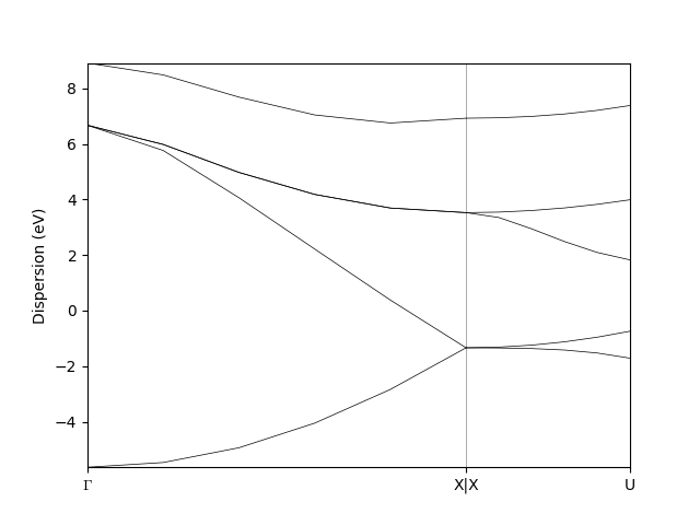
bs.show_mpl() # to visualize the bands
The resulting band structure will look as follows
Warning
Once the bs object is stored (bs.store()) – it won’t
accept any modifications.
Plotting the band structure
You may notice that depending on how you assign the kpoints labels the output
of the show_mpl() method looks different. Please compare:
bs.labels = [(0, 'GAMMA'),
          (5, 'X'),
          (6, 'Y'),
          (11, 'U')]
bs.show_mpl()

bs.labels = [(0, 'GAMMA'),
          (5, 'X'),
          (7, 'Y'),
          (11, 'U')]
bs.show_mpl()
In the first case two neighboring kpoints with X and Y labels will look like
X|Y, while in the second case they will be separated by a certain distance.
The logic behind such a difference is the following. In the first case the
plotting method discovers the two neighboring kpoints and assumes them to be a
discontinuity point in the band structure (e.g. Gamma-X|Y-U). In the second case the
kpoints labelled X and Y are not neighbors anymore, so they are
plotted with a certain distance between them. The intervals between the kpoints on the X axis are
proportional to the cartesian distance between them.
Dealing with spins
The BandsData object can also deal with the results of spin-polarized calculations. Two
provide different bands for two different spins you should just merge them in
one array and import them again using the set_bands() method:
bands_spins = [bands, bands-0.3] # to distinguish the bands of different spins we substitute 0.3 from the second band structure
bs.set_bands(bands_spins, units='eV')
bs.show_mpl()
Now the shape of the bands array becomes nspins * nkpoints * nstates