Basic tutorial

The goal of this tutorial is to give you an idea of how AiiDA helps you in executing data-driven workflows. At the end of this tutorial, you will know how to:

• Store data in the database and subsequently retrieve it.

• Decorate a Python function such that its inputs and outputs are automatically tracked.

• Run and monitor the status of processes.

• Explore and visualize the provenance graph.

Important

If you are working on your own machine, note that the tutorial assumes that you have a working AiiDA installation and have set up your AiiDA profile in the current Python environment. If this is not the case, consult the getting started page.

Important

If you are running this tutorial in a Jupyter notebook, make sure to call load_profile() in a separate cell before running any AiiDA engine processes (e.g. calculation functions or work chains).

Tip

This tutorial can be downloaded and run as a Jupyter Notebook: basic.ipynb

Show code cell content Hide code cell content

from aiida import load_profile, engine, orm, plugins
from aiida.manage.configuration import get_config
from aiida.storage.sqlite_temp import SqliteTempBackend

%load_ext aiida

profile = load_profile(
    SqliteTempBackend.create_profile(
        'myprofile',
        options={
            'warnings.development_version': False,
            'runner.poll.interval': 1
        },
        debug=False
    ),
    allow_switch=True
)
config = get_config()
config.add_profile(profile)
config.set_default_profile(profile.name)
profile

Profile<uuid='10ad077a9c46404da0a6ac300d07a148' name='myprofile'>

Provenance

Before we dive in, we need to briefly introduce one of the most important concepts for AiiDA: provenance. An AiiDA database does not only contain the results of your calculations, but also their inputs and each step that was executed to obtain them. All of this information is stored in the form of a directed acyclic graph (DAG). As an example, Fig. 1 shows the provenance of the calculations of this tutorial.

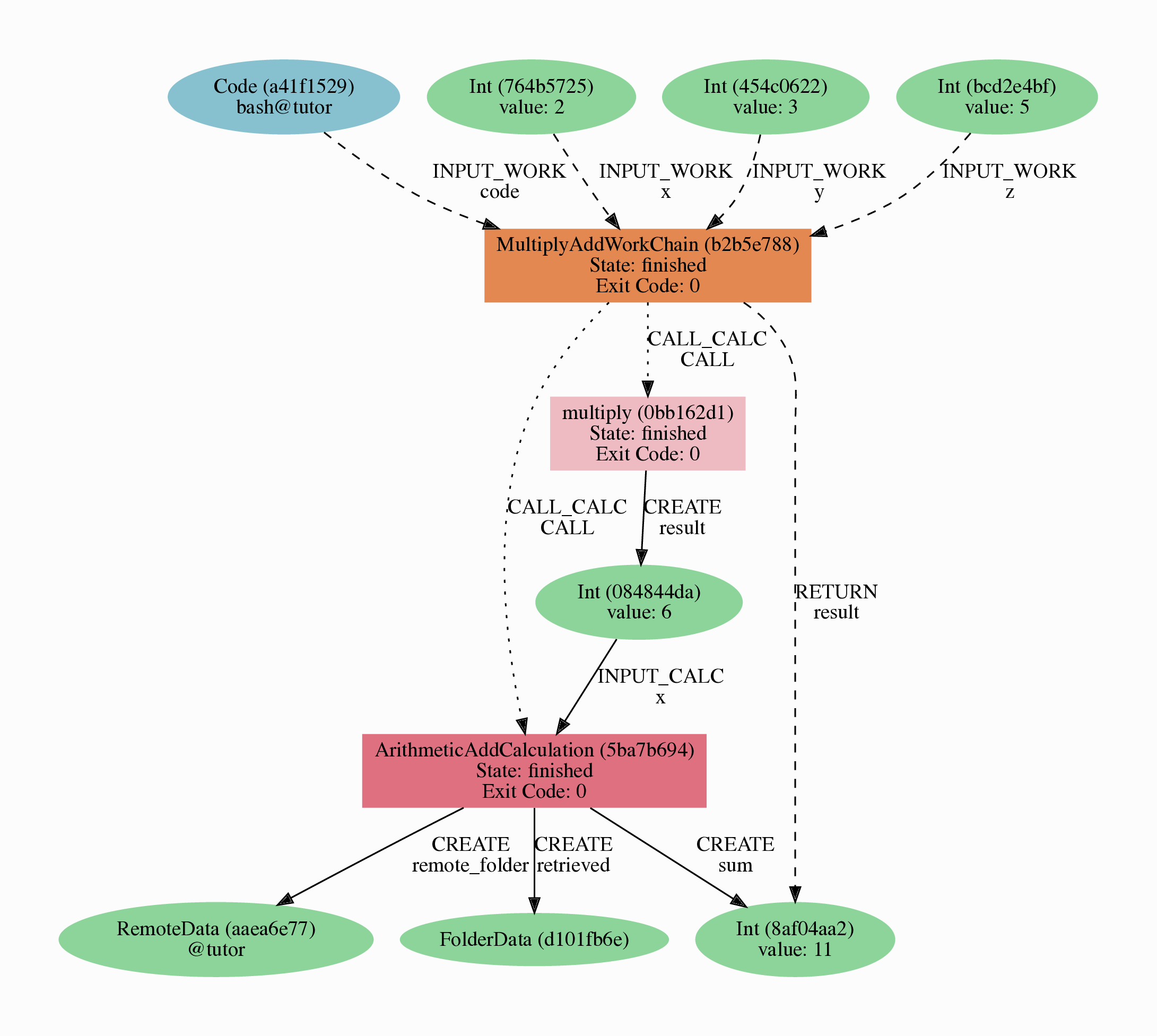
Fig. 1 Provenance Graph of a basic AiiDA WorkChain.

In the provenance graph, you can see different types of nodes represented by different shapes. The green ellipses are Data nodes, the blue ellipse is a Code node, and the rectangles represent processes, i.e. the calculations performed in your workflow.

The provenance graph allows us to not only see what data we have, but also how it was produced. During this tutorial, we will be using AiiDA to generate the provenance graph in Fig. 1 step by step.

Data nodes

Before running any calculations, let’s create and store a data node. AiiDA ships with an interactive IPython shell that has many basic AiiDA classes pre-loaded. To start the IPython shell, simply type in the terminal:

$ verdi shell

AiiDA implements data node types for the most common types of data (int, float, str, etc.), which you can extend with your own (composite) data node types if needed. For this tutorial, we’ll keep it very simple, and start by initializing an Int node and assigning it to the node variable:

from aiida import orm

node = orm.Int(2)

We can check the contents of the node variable like this:

node

<Int: uuid: 1c5cbd60-e003-40d8-8ffa-968dae2b18ea (unstored) value: 2>

Quite a bit of information on our freshly created node is returned:

• The data node is of the type Int

• The node has the universally unique identifier (UUID) eac48d2b-ae20-438b-aeab-2d02b69eb6a8

• The node is currently not stored in the database (unstored)

• The integer value of the node is 2

Let’s store the node in the database:

node.store()

<Int: uuid: 1c5cbd60-e003-40d8-8ffa-968dae2b18ea (pk: 1) value: 2>

As you can see, the data node has now been assigned a primary key (PK), a number that identifies the node in your database (pk: 1). The PK and UUID both reference the node with the only difference that the PK is unique for your local database only, whereas the UUID is a globally unique identifier and can therefore be used between different databases. Use the PK only if you are working within a single database, i.e. in an interactive session and the UUID in all other cases.

Important

The PK numbers shown throughout this tutorial assume that you start from a completely empty database. It is possible that the nodes’ PKs will be different for your database!

The UUIDs are generated randomly and are, therefore, guaranteed to be different.

Next, let’s leave the IPython shell by typing exit() and then enter. Back in the terminal, use the verdi command line interface (CLI) to check the data node we have just created:

%verdi node show 1

Property     Value
-----------  ------------------------------------
type         Int
pk           1
uuid         1c5cbd60-e003-40d8-8ffa-968dae2b18ea
label
description
ctime        2026-06-02 11:55:05.289812+00:00
mtime        2026-06-02 11:55:05.326338+00:00

Once again, we can see that the node is of type Int, has PK = 1, and UUID = eac48d2b-ae20-438b-aeab-2d02b69eb6a8. Besides this information, the verdi node show command also shows the (empty) label and description, as well as the time the node was created (ctime) and last modified (mtime).

Note

AiiDA already provides many standard data types, but you can also create your own.

Calculation functions

Once your data is stored in the database, it is ready to be used for some computational task. For example, let’s say you want to multiply two Int data nodes. The following Python function:

def multiply(x, y):
    return x * y

will give the desired result when applied to two Int nodes, but the calculation will not be stored in the provenance graph. However, we can use a Python decorator provided by AiiDA to automatically make it part of the provenance graph. Start up the AiiDA IPython shell again using verdi shell and execute the following code snippet:

from aiida import engine

@engine.calcfunction
def multiply(x, y):
    return x * y

This converts the multiply function into an AiiDA calculation function, the most basic execution unit in AiiDA. Next, load the Int node you have created in the previous section using the load_node function and the PK of the data node:

x = orm.load_node(pk=1)

Of course, we need another integer to multiply with the first one. Let’s create a new Int data node and assign it to the variable y:

y = orm.Int(3)

Now it’s time to multiply the two numbers!

multiply(x, y)

<Int: uuid: 740b7099-bd64-4222-97cd-094dfcdcaa99 (pk: 4) value: 6>

Success! The calcfunction-decorated multiply function has multiplied the two Int data nodes and returned a new Int data node whose value is the product of the two input nodes. Note that by executing the multiply function, all input and output nodes are automatically stored in the database:

y

<Int: uuid: 6b4118d0-4c67-4334-a919-e8d5af8f24ab (pk: 2) value: 3>

We had not yet stored the data node assigned to the y variable, but by providing it as an input argument to the multiply function, it was automatically stored with PK = 2. Similarly, the returned Int node with value 6 has been stored with PK = 4.

Let’s once again leave the IPython shell with exit() and look for the process we have just run using the verdi CLI:

%verdi process list

PK    Created    Process label    ♻    Process State    Process status
----  ---------  ---------------  ---  ---------------  ----------------

Total results: 0

Report: ♻ Processes marked with check-mark were not run but taken from the cache.
Report: Add the option `-P pk cached_from` to the command to display cache source.
Report: Last time an entry changed state: 0s ago (at 11:55:05 on 2026-06-02)
Warning: This profile does not have a broker and so it has no daemon. See https://aiida-core.readthedocs.io/en/stable/installation/guide_quick.html#quick-install-limitations

The returned list will be empty, but don’t worry! By default, verdi process list only returns the active processes. If you want to see all processes (i.e. also the processes that are terminated), simply add the -a option:

%verdi process list -a

  PK  Created    Process label    ♻    Process State    Process status
----  ---------  ---------------  ---  ---------------  ----------------
   3  0s ago     multiply              ⏹ Finished [0]

Total results: 1

Report: ♻ Processes marked with check-mark were not run but taken from the cache.
Report: Add the option `-P pk cached_from` to the command to display cache source.
Report: Last time an entry changed state: 0s ago (at 11:55:05 on 2026-06-02)
Warning: This profile does not have a broker and so it has no daemon. See https://aiida-core.readthedocs.io/en/stable/installation/guide_quick.html#quick-install-limitations

We can see that our multiply calcfunction was created 1 minute ago, assigned the PK 3, and has Finished.

As a final step, let’s have a look at the provenance of this simple calculation. The provenance graph can be automatically generated using the verdi CLI. Let’s generate the provenance graph for the multiply calculation function we have just run with PK = 3:

$ verdi node graph generate 3

The command will write the provenance graph to a .pdf file. Use your favorite PDF viewer to have a look. It should look something like the graph shown below.

Show code cell source Hide code cell source

from aiida.tools.visualization import Graph
graph = Graph()
calc_node = orm.load_node(3)
graph.add_incoming(calc_node, annotate_links="both")
graph.add_outgoing(calc_node, annotate_links="both")
graph.graphviz

Fig. 2 Provenance graph of the multiply calculation function.

Note

Remember that the PK of the calcfunction can be different for your database.

CalcJobs

When running calculations that require an external code or run on a remote machine, a simple calculation function is no longer sufficient. For this purpose, AiiDA provides the CalcJob process class.

To run a CalcJob, you need to set up two things: a code that is going to implement the desired calculation and a computer for the calculation to run on.

If you’re running this tutorial in the Quantum Mobile VM or on Binder, these have been pre-configured for you. If you’re running on your own machine, you can follow the instructions in the panel below.

See also

More details for how to run external codes.

Install localhost computer and code

Let’s begin by setting up the computer using the verdi computer subcommand:

$ verdi computer setup -L tutor -H localhost -T core.local -S core.direct -w `echo $PWD/work` -n
$ verdi computer configure core.local tutor --safe-interval 1 -n

The first commands sets up the computer with the following options:

• label (-L): tutor

• hostname (-H): localhost

• transport (-T): local

• scheduler (-S): direct

• work-dir (-w): The work subdirectory of the current directory

The second command configures the computer with a minimum interval between connections (--safe-interval) of 1 second. For both commands, the non-interactive option (-n) is added to not prompt for extra input.

Next, let’s set up the code we’re going to use for the tutorial:

$ verdi code create core.code.installed --label add --computer=tutor --default-calc-job-plugin core.arithmetic.add --filepath-executable=/bin/bash -n

This command sets up a code with label add on the computer tutor, using the plugin core.arithmetic.add.

Show code cell content Hide code cell content

%verdi computer setup -L tutor -H localhost -T core.local -S core.direct -w /tmp -n
%verdi computer configure core.local tutor --safe-interval 0 -n
%verdi code create core.code.installed --label add --computer=tutor --default-calc-job-plugin core.arithmetic.add --filepath-executable=/bin/bash -n

Success: Computer<1> tutor created
Report: Note: before the computer can be used, it has to be configured with the command:
Report:   verdi -p myprofile computer configure core.local tutor
Report: Configuring computer tutor for user user@email.com.
Success: tutor successfully configured for user@email.com
Success: Created InstalledCode<5>

A typical real-world example of a computer is a remote supercomputing facility. Codes can be anything from a Python script to powerful ab initio codes such as Quantum Espresso or machine learning tools like Tensorflow. Let’s have a look at the codes that are available to us:

%verdi code list

Full label      Pk  Entry point
------------  ----  -------------------
add@tutor        5  core.code.installed

Use `verdi code show IDENTIFIER` to see details for a code

You can see a single code add@tutor, with PK = 5, in the printed list. This code allows us to add two integers together. The add@tutor identifier indicates that the code with label add is run on the computer with label tutor. To see more details about the computer, you can use the following verdi command:

%verdi computer show tutor

---------------------------  ------------------------------------
Label                        tutor
PK                           1
UUID                         d5819023-9872-4702-b0e7-47d7d1d97ec8
Description
Hostname                     localhost
Transport type               core.local
Scheduler type               core.direct
Work directory               /tmp
Shebang                      #!/bin/bash
Mpirun command               mpirun -np {tot_num_mpiprocs}
Default #procs/machine
Default memory (kB)/machine
Prepend text
Append text
---------------------------  ------------------------------------

We can see that the Work directory has been set up as the work subdirectory of the current directory. This is the directory in which the calculations running on the tutor computer will be executed.

Note

You may have noticed that the PK of the tutor computer is 1, same as the Int node we created at the start of this tutorial. This is because different entities, such as nodes, computers and groups, are stored in different tables of the database. So, the PKs for each entity type are unique for each database, but entities of different types can have the same PK within one database.

Let’s now start up the verdi shell again and load the add@tutor code using its label:

code = orm.load_code(label='add')
code

<InstalledCode: Remote code 'add' on tutor pk: 5, uuid: df67fbab-9fc1-4a40-a4cd-fec95e1c3731>

Every code has a convenient tool for setting up the required input, called the builder. It can be obtained by using the get_builder method:

builder = code.get_builder()
builder

Process class: ArithmeticAddCalculation
Inputs:
code: add@tutor

Using the builder, you can easily set up the calculation by directly providing the input arguments. Let’s use the Int node that was created by our previous calcfunction as one of the inputs and a new node as the second input:

builder.x = orm.load_node(pk=4)
builder.y = orm.Int(5)
builder

Process class: ArithmeticAddCalculation
Inputs:
code: add@tutor
x: 6
y: 5

In case that your nodes’ PKs are different and you don’t remember the PK of the output node from the previous calculation, check the provenance graph you generated earlier and use the UUID of the output node instead:

In [3]: builder.x = orm.load_node(uuid='42541d38')
   ...: builder.y = orm.Int(5)

Note that you don’t have to provide the entire UUID to load the node. As long as the first part of the UUID is unique within your database, AiiDA will find the node you are looking for.

Note

One nifty feature of the builder is the ability to use tab completion for the inputs. Try it out by typing builder. + <TAB> in the verdi shell.

To execute the CalcJob, we use the run function provided by the AiiDA engine, and wait for the process to complete:

engine.run(builder)

{'remote_folder': <RemoteData: uuid: 807a3372-aaa0-441e-9a3d-55951f0ad858 (pk: 8)>,
 'retrieved': <FolderData: uuid: e3bf0f85-d5d2-4ceb-aedd-a8f08d54cc31 (pk: 9)>,
 'sum': <Int: uuid: 79eb9faa-ecaf-4100-abd7-e28792f2a4d8 (pk: 10) value: 11>}

Besides the sum of the two Int nodes, the calculation function also returns two other outputs: one of type RemoteData and one of type FolderData. See the topics section on calculation jobs for more details. Now, exit the IPython shell and once more check for all processes:

%verdi process list -a

  PK  Created    Process label             ♻    Process State    Process status
----  ---------  ------------------------  ---  ---------------  ----------------
   3  1s ago     multiply                       ⏹ Finished [0]
   7  0s ago     ArithmeticAddCalculation       ⏹ Finished [0]

Total results: 2

Report: ♻ Processes marked with check-mark were not run but taken from the cache.
Report: Add the option `-P pk cached_from` to the command to display cache source.
Report: Last time an entry changed state: 0s ago (at 11:55:06 on 2026-06-02)
Warning: This profile does not have a broker and so it has no daemon. See https://aiida-core.readthedocs.io/en/stable/installation/guide_quick.html#quick-install-limitations

You should now see two processes in the list. One is the multiply calcfunction you ran earlier, the second is the ArithmeticAddCalculation CalcJob that you have just run. Grab the PK of the ArithmeticAddCalculation, and generate the provenance graph. The result should look like the graph shown below.

$ verdi node graph generate 7

Show code cell source Hide code cell source

from aiida.tools.visualization import Graph
graph = Graph()
calc_node = orm.load_node(7)
graph.recurse_ancestors(calc_node, annotate_links="both")
graph.add_outgoing(calc_node, annotate_links="both")
graph.graphviz

You can see more details on any process, including its inputs and outputs, using the verdi shell:

%verdi process show 7

Property     Value
-----------  ------------------------------------
type         ArithmeticAddCalculation
state        Finished [0]
pk           7
uuid         9e9e20f2-7021-4fcd-8abb-4c24ed6206aa
label
description
ctime        2026-06-02 11:55:06.200125+00:00
mtime        2026-06-02 11:55:06.840180+00:00
computer     [1] tutor

Inputs      PK  Type
--------  ----  -------------
code         5  InstalledCode
x            4  Int
y            6  Int

Outputs          PK  Type
-------------  ----  ----------
remote_folder     8  RemoteData
retrieved         9  FolderData
sum              10  Int

Workflows

So far we have executed each process manually. AiiDA allows us to automate these steps by linking them together in a workflow, whose provenance is stored to ensure reproducibility. For this tutorial we have prepared a basic WorkChain that is already implemented in aiida-core. You can see the code below:

MultiplyAddWorkChain code

"""Implementation of the MultiplyAddWorkChain for testing and demonstration purposes."""

from aiida.calculations.arithmetic.add import ArithmeticAddCalculation
from aiida.engine import ToContext, WorkChain, calcfunction
from aiida.orm import AbstractCode, Int


@calcfunction
def multiply(x, y):
    return x * y


class MultiplyAddWorkChain(WorkChain):
    """WorkChain to multiply two numbers and add a third, for testing and demonstration purposes."""

    @classmethod
    def define(cls, spec):
        """Specify inputs and outputs."""
        super().define(spec)
        spec.input('x', valid_type=Int)
        spec.input('y', valid_type=Int)
        spec.input('z', valid_type=Int)
        spec.input('code', valid_type=AbstractCode)
        spec.outline(
            cls.multiply,
            cls.add,
            cls.validate_result,
            cls.result,
        )
        spec.output('result', valid_type=Int)
        spec.exit_code(400, 'ERROR_NEGATIVE_NUMBER', message='The result is a negative number.')

    def multiply(self):
        """Multiply two integers."""
        self.ctx.product = multiply(self.inputs.x, self.inputs.y)

    def add(self):
        """Add two numbers using the `ArithmeticAddCalculation` calculation job plugin."""
        inputs = {'x': self.ctx.product, 'y': self.inputs.z, 'code': self.inputs.code}
        future = self.submit(ArithmeticAddCalculation, **inputs)
        self.report(f'Submitted the `ArithmeticAddCalculation`: {future}')
        return ToContext(addition=future)

    def validate_result(self):
        """Make sure the result is not negative."""
        result = self.ctx.addition.outputs.sum

        if result.value < 0:
            return self.exit_codes.ERROR_NEGATIVE_NUMBER

    def result(self):
        """Add the result to the outputs."""
        self.out('result', self.ctx.addition.outputs.sum)

First, we recognize the multiply function we have used earlier, decorated as a calcfunction. The define class method specifies the input and output of the WorkChain, as well as the outline, which are the steps of the workflow. These steps are provided as methods of the MultiplyAddWorkChain class.

Show code cell content Hide code cell content

from aiida.engine import ToContext, WorkChain, calcfunction
from aiida.orm import AbstractCode, Int
from aiida.plugins.factories import CalculationFactory

ArithmeticAddCalculation = CalculationFactory('core.arithmetic.add')


@calcfunction
def multiply(x, y):
    return x * y


class MultiplyAddWorkChain(WorkChain):
    """WorkChain to multiply two numbers and add a third, for testing and demonstration purposes."""

    @classmethod
    def define(cls, spec):
        """Specify inputs and outputs."""
        super().define(spec)
        spec.input('x', valid_type=Int)
        spec.input('y', valid_type=Int)
        spec.input('z', valid_type=Int)
        spec.input('code', valid_type=AbstractCode)
        spec.outline(
            cls.multiply,
            cls.add,
            cls.validate_result,
            cls.result,
        )
        spec.output('result', valid_type=Int)
        spec.exit_code(400, 'ERROR_NEGATIVE_NUMBER', message='The result is a negative number.')

    def multiply(self):
        """Multiply two integers."""
        self.ctx.product = multiply(self.inputs.x, self.inputs.y)

    def add(self):
        """Add two numbers using the `ArithmeticAddCalculation` calculation job plugin."""
        inputs = {'x': self.ctx.product, 'y': self.inputs.z, 'code': self.inputs.code}
        future = self.submit(ArithmeticAddCalculation, **inputs)

        return ToContext(addition=future)

    def validate_result(self):
        """Make sure the result is not negative."""
        result = self.ctx.addition.outputs.sum

        if result.value < 0:
            return self.exit_codes.ERROR_NEGATIVE_NUMBER

    def result(self):
        """Add the result to the outputs."""
        self.out('result', self.ctx.addition.outputs.sum)

Note

Besides WorkChains, workflows can also be implemented as work functions. These are ideal for workflows that are not very computationally intensive and can be easily implemented in a Python function.

Let’s run the WorkChain above!

Start up the verdi shell and load the MultiplyAddWorkChain using the WorkflowFactory:

from aiida import plugins
MultiplyAddWorkChain = plugins.WorkflowFactory('core.arithmetic.multiply_add')

The WorkflowFactory loads workflows based on their entry point, e.g. 'core.arithmetic.multiply_add' in this case. The entry point mechanism allows AiiDA to automatically discover workflows provided by aiida-core and AiiDA plugins, and display them to the user, e.g. via verdi plugin list aiida.workflows. Pass the entry point as an argument to display detailed information, e.g. via verdi plugin list aiida.workflows core.arithmetic.multiply_add.

Similar to a CalcJob, the WorkChain input can be set up using a builder:

from aiida import orm
builder = MultiplyAddWorkChain.get_builder()
builder.code = orm.load_code(label='add')
builder.x = orm.Int(2)
builder.y = orm.Int(3)
builder.z = orm.Int(5)
builder

Process class: MultiplyAddWorkChain
Inputs:
code: add@tutor
x: 2
y: 3
z: 5

Once the WorkChain input has been set up, we run it with the AiiDA engine:

from aiida import engine
engine.run(builder)

Report: [14|MultiplyAddWorkChain|add]: Submitted the `ArithmeticAddCalculation`: uuid: a2fa8643-58b9-40b5-92ee-312305c5427b (pk: 17) (aiida.calculations:core.arithmetic.add)

{'result': <Int: uuid: 3fdda387-3df0-4eb1-8753-ac62b06d944e (pk: 20) value: 11>}

Now quickly leave the IPython shell and check the process list:

%verdi process list -a

  PK  Created    Process label             ♻    Process State    Process status
----  ---------  ------------------------  ---  ---------------  ----------------
   3  3s ago     multiply                       ⏹ Finished [0]
   7  2s ago     ArithmeticAddCalculation       ⏹ Finished [0]
  14  1s ago     MultiplyAddWorkChain           ⏹ Finished [0]
  15  1s ago     multiply                       ⏹ Finished [0]
  17  1s ago     ArithmeticAddCalculation       ⏹ Finished [0]

Total results: 5

Report: ♻ Processes marked with check-mark were not run but taken from the cache.
Report: Add the option `-P pk cached_from` to the command to display cache source.
Report: Last time an entry changed state: 0s ago (at 11:55:08 on 2026-06-02)
Warning: This profile does not have a broker and so it has no daemon. See https://aiida-core.readthedocs.io/en/stable/installation/guide_quick.html#quick-install-limitations

Submitting to the daemon

If instead we had submitted to the daemon (see Submitting to the daemon), we would see the the process status of the workchain and its dependants:

$ verdi process list -a
  PK  Created    Process label             Process State    Process status
----  ---------  ------------------------  ---------------  ------------------------------------
   3  7m ago     multiply                  ⏹ Finished [0]
   7  3m ago     ArithmeticAddCalculation  ⏹ Finished [0]
  12  2m ago     ArithmeticAddCalculation  ⏹ Finished [0]
  19  16s ago    MultiplyAddWorkChain      ⏵ Waiting        Waiting for child processes: 22
  20  16s ago    multiply                  ⏹ Finished [0]
  22  15s ago    ArithmeticAddCalculation  ⏵ Waiting        Waiting for transport task: retrieve

Total results: 6

Info: last time an entry changed state: 0s ago (at 09:08:59 on 2020-05-13)

We can see that the MultiplyAddWorkChain is currently waiting for its child process, the ArithmeticAddCalculation, to finish. Check the process list again for all processes (You should know how by now!). After about half a minute, all the processes should be in the Finished state. The verdi process status command prints a hierarchical overview of the processes called by the work chain:

%verdi process status 14

MultiplyAddWorkChain<14> Finished [0] [3:result]
    ├── multiply<15> Finished [0]
    └── ArithmeticAddCalculation<17> Finished [0]

The bracket [3:result] indicates the current step in the outline of the MultiplyAddWorkChain (step 3, with name result). The process status is particularly useful for debugging complex work chains, since it helps pinpoint where a problem occurred.

We can now generate the full provenance graph for the WorkChain with:

$ verdi node graph generate 14

Show code cell source Hide code cell source

from aiida.tools.visualization import Graph
graph = Graph()
calc_node = orm.load_node(14)
graph.recurse_ancestors(calc_node, annotate_links="both")
graph.recurse_descendants(calc_node, annotate_links="both")
graph.graphviz

Look familiar? The provenance graph should be similar to the one we showed at the start of this tutorial (Fig. 1).

Submitting to the daemon

When we used the run command in the previous sections, the IPython shell was blocked while it was waiting for the CalcJob to finish. This is not a problem when we’re simply adding two number together, but if we want to run multiple calculations that take hours or days, this is no longer practical. Instead, we are going to submit the CalcJob to the AiiDA daemon. The daemon is a program that runs in the background and manages submitted calculations until they are terminated. Let’s first check the status of the daemon using the verdi CLI:

$ verdi daemon status

If the daemon is running, the output will be something like the following:

Profile: tutorial
Daemon is running as PID 96447 since 2020-05-22 18:04:39
Active workers [1]:
  PID    MEM %    CPU %  started
-----  -------  -------  -------------------
96448    0.507        0  2020-05-22 18:04:39
Use verdi daemon [incr | decr] [num] to increase / decrease the amount of workers

In this case, let’s stop it for now:

$ verdi daemon stop

Next, let’s submit the CalcJob we ran previously. Start the verdi shell and execute the Python code snippet below. This follows all the steps we did previously, but now uses the submit function instead of run:

In [1]: from aiida.engine import submit
   ...:
   ...: code = load_code(label='add')
   ...: builder = code.get_builder()
   ...: builder.x = load_node(pk=4)
   ...: builder.y = Int(5)
   ...:
   ...: submit(builder)

When using submit the calculation job is not run in the local interpreter but is sent off to the daemon and you get back control instantly. Instead of the result of the calculation, it returns the node of the CalcJob that was just submitted:

Out[1]: <CalcJobNode: uuid: e221cf69-5027-4bb4-a3c9-e649b435393b (pk: 12) (aiida.calculations:core.arithmetic.add)>

Let’s exit the IPython shell and have a look at the process list:

$ verdi process list

You should see the CalcJob you have just submitted, with the state Created:

  PK  Created    Process label             Process State    Process status
----  ---------  ------------------------  ---------------  ----------------
  12  13s ago    ArithmeticAddCalculation  ⏹ Created

Total results: 1

Info: last time an entry changed state: 13s ago (at 09:06:57 on 2020-05-13)

The CalcJob process is now waiting to be picked up by a daemon runner, but the daemon is currently disabled. Let’s start it up (again):

$ verdi daemon start

Now you can either use verdi process list to follow the execution of the CalcJob, or watch its progress:

$ verdi process watch 12

Let’s wait for the CalcJob to complete and then use verdi process list -a to see all processes we have run so far:

  PK  Created    Process label             Process State    Process status
----  ---------  ------------------------  ---------------  ----------------
   3  6m ago     multiply                  ⏹ Finished [0]
   7  2m ago     ArithmeticAddCalculation  ⏹ Finished [0]
  12  1m ago     ArithmeticAddCalculation  ⏹ Finished [0]

Total results: 3

Info: last time an entry changed state: 14s ago (at 09:07:45 on 2020-05-13)

Next Steps

Congratulations! You have completed the first step to becoming an AiiDA expert.

We have compiled how-to guides that are especially relevant for the following use cases:

Run pure Python lightweight computations

Designing a workflow

After reading the Basic Tutorial, you may want to learn about how to encode the logic of a typical scientific workflow in the writing workflows how-to.

Reusable data types

If you have a certain input or output data type, which you use often, then you may wish to turn it into its own data plugin.

Finding and querying for your data

Once you have run multiple computations, the find and query data how-to can show you how to efficiently explore your data. The data lineage can also be visualised as a provenance graph.

Sharing your data

You can export all or part of your data to file with the export/import functionality or you can even serve your data over HTTP(S) using the AiiDA REST API.

Sharing your workflows

Once you have a working computation workflow, you may also wish to package it into a python module for others to use.

Run compute-intensive codes

Working with external codes

Existing calculation plugins, for interfacing with external codes, are available on the aiida plugin registry. If none meet your needs, then the external codes how-to can show you how to create your own calculation plugin.

Tuning performance

To optimise the performance of AiiDA for running many concurrent computations see the tuning performance how-to.

Saving computational resources

AiiDA can cache and reuse the outputs of identical computations, as described in the caching how-to.

Run computations on High Performance Computers

Connecting to supercomputers

To setup up a computer which can communicate with a high-performance computer over SSH, see the how-to for running external codes, or add a custom transport. AiiDA has pre-written scheduler plugins to work with LSF, PBSPro, SGE, Slurm and Torque.

Working with external codes

Existing calculation plugins, for interfacing with external codes, are available on the aiida plugin registry. If none meet your needs, then the external codes how-to can show you how to create your own calculation plugin.

Exploring your data

Once you have run multiple computations, the find and query data how-to can show you how to efficiently explore your data. The data lineage can also be visualised as a provenance graph.

Sharing your data

You can export all or part of your data to file with the export/import functionality or you can even serve your data over HTTP(S) using the AiiDA REST API.

Sharing your calculation plugin

Once you have a working plugin, you may also wish to package it into a python module for others to use.